System Earth 1b
A planet in and out of equilibrium
Misha Velthuis
m.velthuis@uva.nl
Fri 6 Sept 2024
Recap
Link to recommendations
(Feel free to add/edit!)
Content
Systems thinking
Stocks and flows
Feedback loops
Modeling dynamic equilibria (analytical and numerical)
Perturbations and forcings
Adding features: connected systems + feedback factor
Systems thinking
Tendency to focus on how things connect

Tendency to zoom out
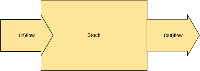
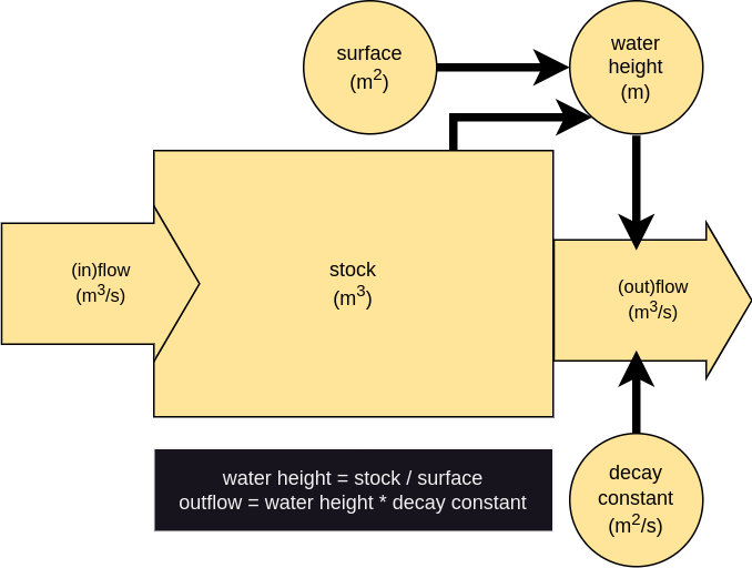
Stocks and flows
Basics
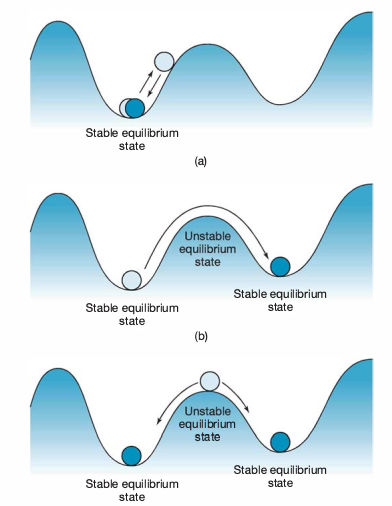
Dynamic equilibria
Average residence time
Average residence time
We are all dynamic equilibria
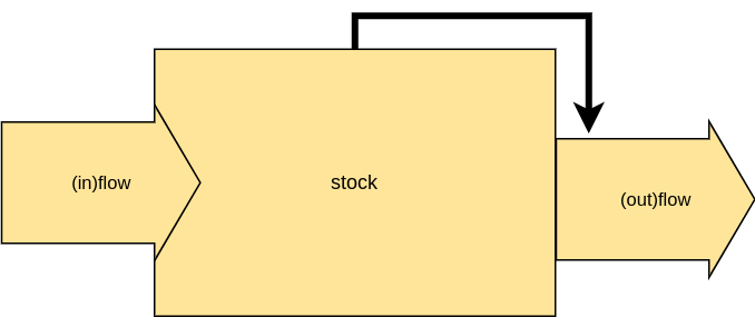
Stocks influencing flows

Me adjusting how much I eat per day
on the basis of how much I weigh
Numbers of deaths per year going up
as the population increases
Feedback loops
Positive and negative couplings
Positive feedback loop:
Change A causes change B
which strengthens change A
Negative feedback loop
Change A causes change B,
which dampens change A
Breaking down in couplings
Positive coupling: –>
Negative coupling: –o
Combining couplings
Positive + positive = positive feedback
Positive + negative = negative feedback
Negative + negative = positive feedback
Spiral of love
happiness A –> happiness B
happiness B –> happiness A
Spiral of toxic comparison
happiness A –o happiness B
happiness B –o happiness A
Stability of a weird friendship
happiness A –> happiness B
happiness B –o happiness A
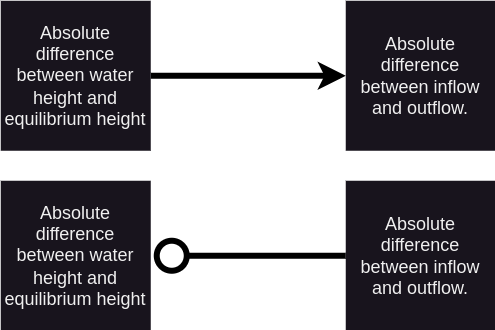
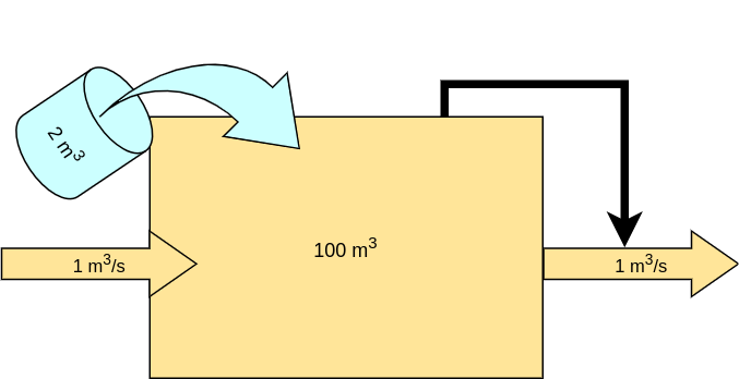
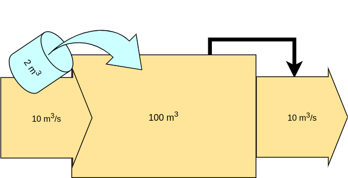
Stability of a reservoir
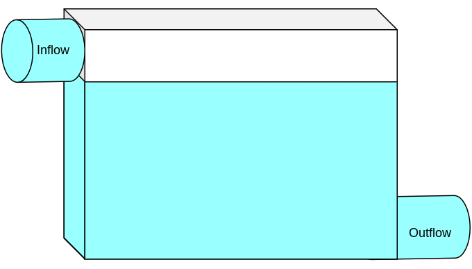
Stability of a reservoir
Recap of (part of) calculus
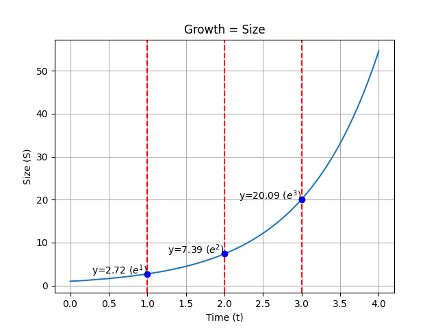
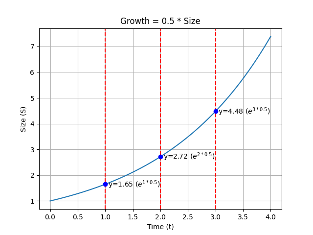
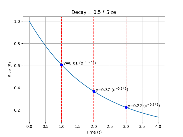
What is Euler's e?
The e of Earth: growth #1
The e of Earth: growth #2
The e of Earth: decay #1
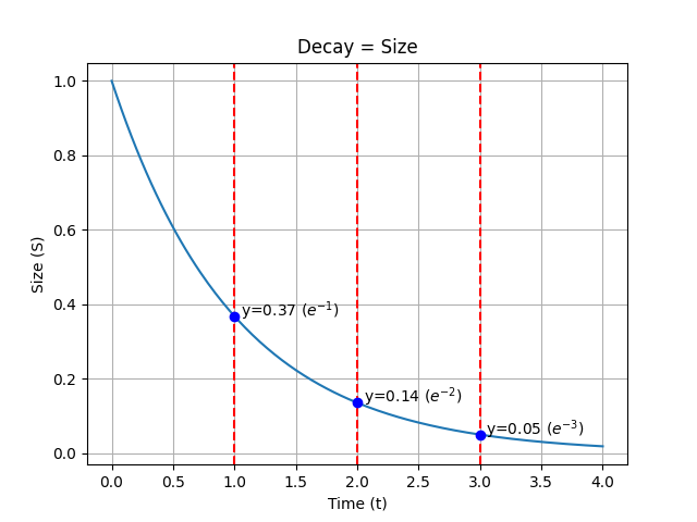
The e of Earth: decay #2
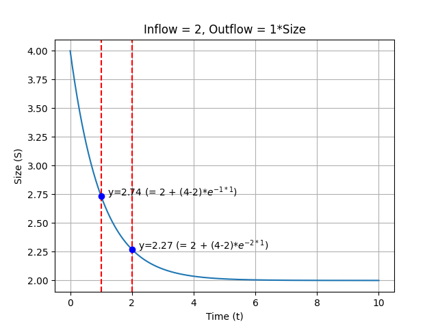
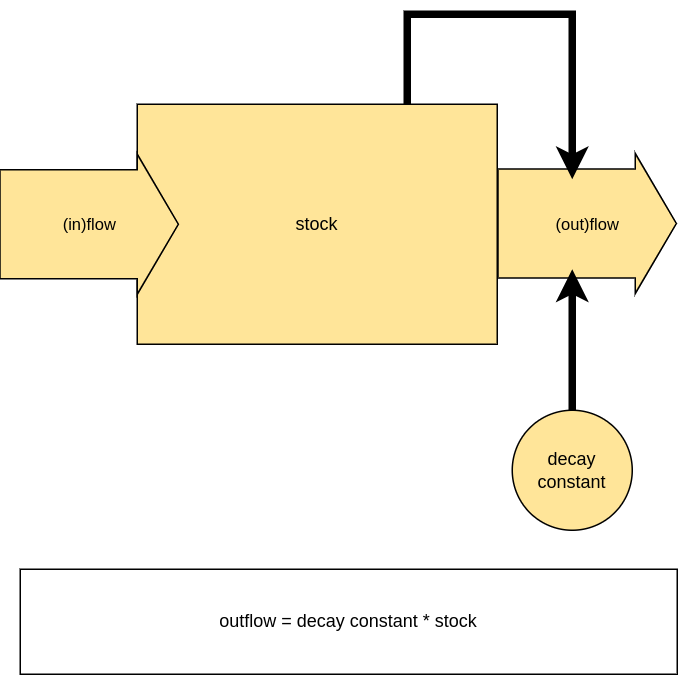
Reservoir: constant inflow, variable outflow
Numerical solutions: the easy way out
Code in Python
# Amount added every timestep
inflow = 2
# Fraction of S that flows out, every timestep
DC = 0.5

# Model runs until this time
t_end=15
# Length of each timestep
dt=1
# Create list of time
time=np.arange(0,t_end,dt)

# Create empy list for numerical series
S_store=[]
# Initialise stock size
S = 6
# For every item in the List time
for t in time:
    # Calculate dS/dt
    dS=inflow-DC*S
    # Multiply dS/dt with dt and add to current stock size
    S=S+(dS*dt)
    # Append the new stock size
    S_store.append(S)
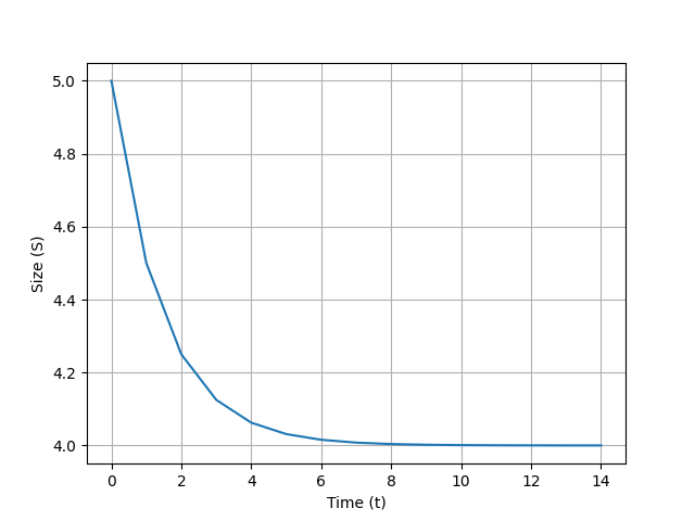
Code in Python with graph
import numpy as np
import matplotlib.pyplot as plt

# Amount added every timestep
inflow = 2
# Fraction of S that flows out, every timestep
DC = 0.5

# Model runs until this time
t_end=15
# Length of each timestep
dt=1
# Create list of time
time=np.arange(0,t_end,dt)

# Create empy list for numerical series
S_store=[]
# Initialise stock size
S = 6
# For every item in the List time
for t in time:
    # Calculate dS/dt
    dS=inflow-DC*S
    # Multiply dS/dt with dt and add to stock size
    S=S+(dS*dt)
    # Append the new stock size
    S_store.append(S)

# PLOTTING
plt.plot(time,S_store)
plt.xlabel('Time (t)')
plt.ylabel('Size (S)')
plt.grid(True)
plt.savefig("/home/misha/Nextcloud/mnotes/mnotes_folders/presentations/images/numerical-example.png")
plt.close()
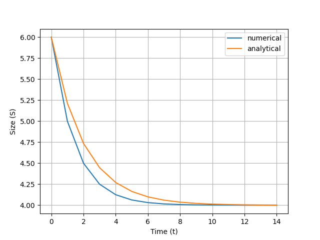
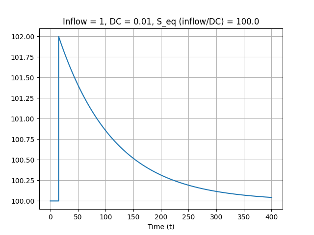
Compare numerical and analytic
import numpy as np
import matplotlib.pyplot as plt

# Amount added every timestep
inflow = 2
# Fraction of S that flows out, every timestep
DC = 0.5

# Model runs until this time
t_end=15
# Length of each timestep
dt=1
# Create list of time
time=np.arange(0,t_end,dt)

# Create empy list for numerical series
S_store=[]
# Initialise stock size
S = 6
# For every item in the List time
for t in time:
    # Calculate dS/dt
    dS=inflow-DC*S
    # Multiply dS/dt with dt and add to stock size
    S=S+(dS*dt)
    # Append the new stock size
    S_store.append(S)

# ANALYTICAL SOLUTION
# Determine equilibrium stock size (at which inflow = outflow)
S_eq = inflow/DC
S_init = 6
# Determine how many times the S_eq above/below the S_eq the S starts
diff_init = (S_init-S_eq)/S_eq
S2=S_eq + diff_init*S_eq*np.e**(-time*DC)
# at t=0, np.E**(0) = 1, so if factor is 1, you get Eq_S - Eq_S which is 0

# PLOTTING
plt.plot(time,S_store,label='numerical')
plt.plot(time,S2,label='analytical')
plt.xlabel('Time (t)')
plt.ylabel('Size (S)')
plt.grid(True)
plt.legend()
plt.savefig("/home/misha/Nextcloud/mnotes/mnotes_folders/presentations/images/numerical-analytic-example.png")
plt.close()
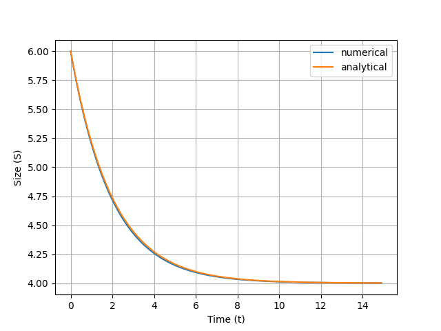
Compare numerical and analytic
import numpy as np
import matplotlib.pyplot as plt

# Amount added every timestep
inflow = 2
# Fraction of S that flows out, every timestep
DC = 0.5

# Model runs until this time
t_end=15
# Length of each timestep
dt=0.1
# Create list of time
time=np.arange(0,t_end,dt)

# Create empy list for numerical series
S_store=[]
# Initialise stock size
S = 6
# For every item in the List time
for t in time:
    # Append the new stock size
    S_store.append(S)
    # Calculate dS/dt
    dS=inflow-DC*S
    # Multiply dS/dt with dt and add to stock size
    S=S+(dS*dt)

# ANALYTICAL SOLUTION
# Determine equilibrium stock size (at which inflow = outflow)
S_eq = inflow/DC
S_init = 6
# Determine how many times the S_eq above/below the S_eq the S starts
diff_init = (S_init-S_eq)/S_eq
S2=S_eq + diff_init*S_eq*np.e**(-time*DC)
# at t=0, np.E**(0) = 1, so if factor is 1, you get Eq_S - Eq_S which is 0

# PLOTTING
plt.plot(time,S_store,label='numerical')
plt.plot(time,S2,label='analytical')
plt.xlabel('Time (t)')
plt.ylabel('Size (S)')
plt.grid(True)
plt.legend()
plt.savefig("/home/misha/Nextcloud/mnotes/mnotes_folders/presentations/images/numerical-analytic-example-small-dt.png")
plt.close()
smaller \(\delta{}t\)
Perturbations and forcings
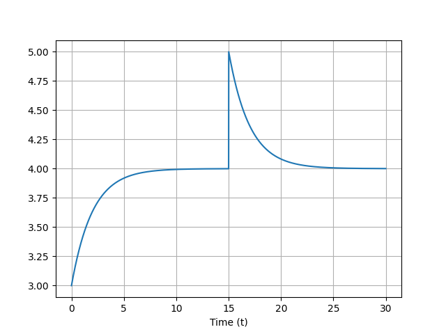 Perturbation
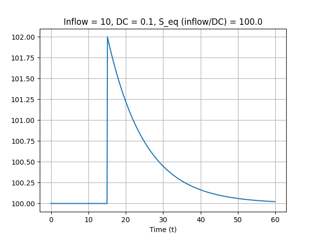
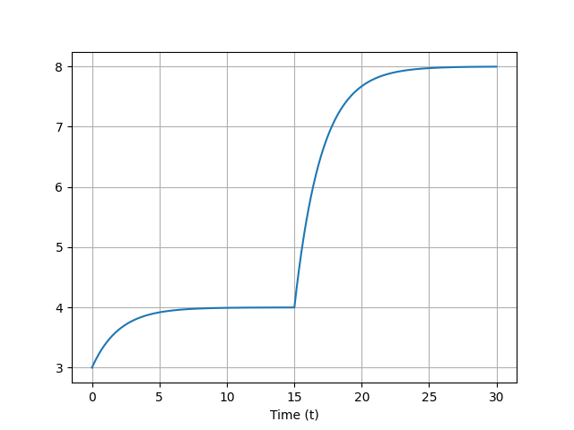 Forcing:
Response time
Let's see …
 Small inflow, relative to equilibrium stock size
Large average residence time
Large response time
 Large inflow, relative to equilibrium stock size
Small average residence time
Small response time
Bottom line …
Dynamic equilibria that have small flows compared to stock sizes (for example because of a small decay constant) have large average residence times, and large response times.
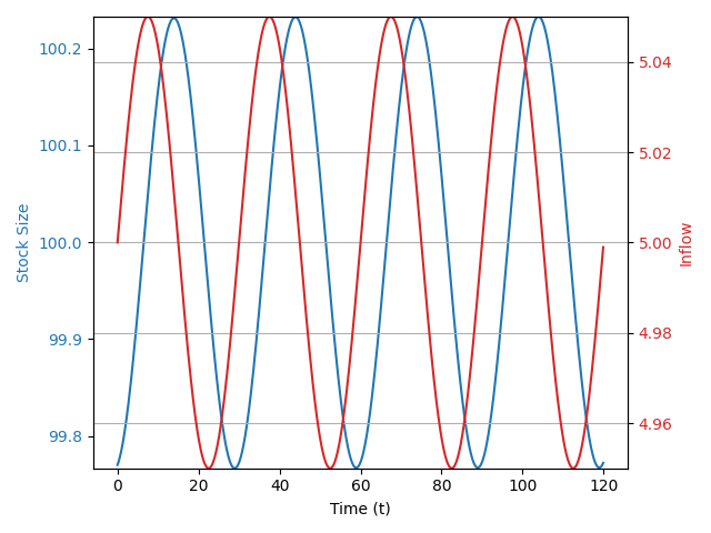
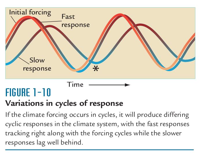
Fluctuating systems
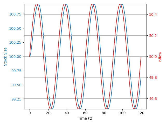
Fluctuations with slower response time
Adding features
Connected systems
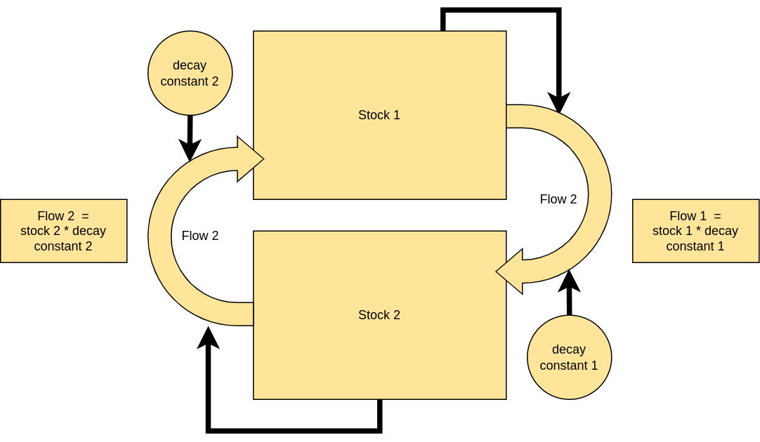
Feedback factors
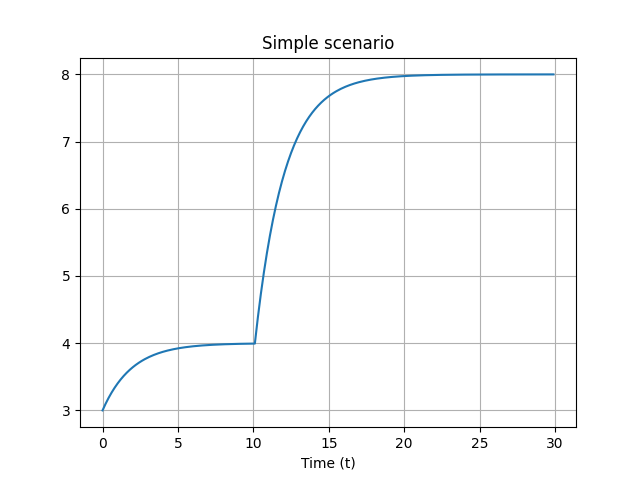
Simple dynamic equilibrium with forcing
Simple dynamic equilibrium with forcing
Simple dynamic equilibrium with forcing
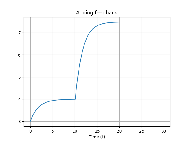
Adding feedback
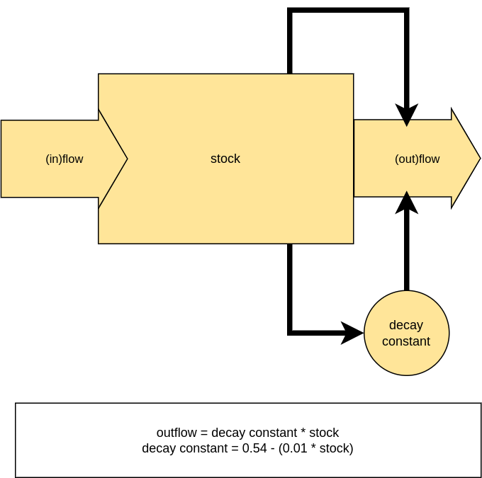
Adding feedback
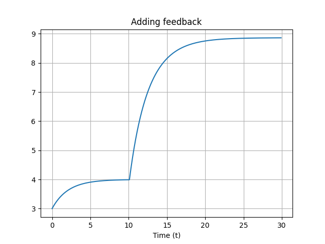
Feedback factor
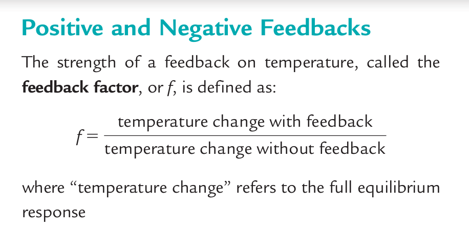
Feedback factor lower than 1
Gaia hypothesis